Category: Amusements

  • sd1diskutil: Resurrecting a disk format from the dead for a brand-new emulator

    A little history

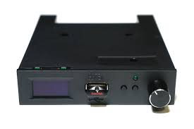
    The Ensoniq SD-1 is a synthesizer from the 1990s — a ROMpler with a Motorola 68000 at its heart. Like many synthesizers of the era, it uses the cheap, easy, and simple storage medium of the day: 800K floppy disks for storage of everything: factory programs, user programs, presets (organized small sets of programs), full-up MIDI sequences, and its own operating system.

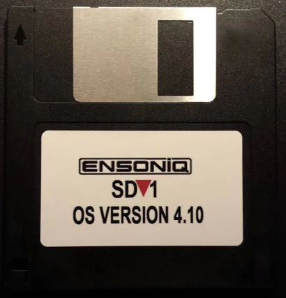
    The format is proprietary and somewhat peculiar: a custom FAT, 10 sectors per track numbered 0 through 9 (not 1 through 10 like a PC), big-endian multi-byte fields throughout, and a handful of file types that the rest of the computing world has never heard of. To retrieve your data on a modern computer, or to get sounds back onto the synth, you need something that can speak this format.

    Few if any USB disk drives can handle this format; the extant programs which can read Ensoniq disks all run under MS-DOS (or Windows DOS emulation) and need a real, wired-in diskette drive to handle reading and writing disks. Forget about doing this on a Mac.

    Fortunately, the SD-1 has a reasonably robust MIDI system-exclusive, or “SysEx”, implementation, capable of dumping and receiving pretty much everything except the actual sequencer OS that can record sequences to the SD-1’s internal memory and play them back. Those of us who saw the handwriting on the wall (and who didn’t want to keep a 486 tower lying around just to write the floppy disks that were becoming harder and harder to find anyway), took the earliest possible opportunity to dump everything out over SysEx and save it elsewhere.

    Getting the sequencer OS back into the thing still needs a diskette, which is an issue (solved by third-party add-ons that could store hundreds of floppy images on a USB stick).

    The renaissance

    But there was some big news in March 2026, that made the question of accessing the SD-1’s disks and data an interesting topic again.

    The folks at Sojus Records announced a wrapper around the previously-created SD-1 MAME emulator that allowed the SD-1 to be loaded as a VST3 plugin.

    For all of us who had SD-1’s (or who still have them, but have shifted to much-more-convenient computer-based sequencing), this was a sit-up-and-take-notice moment. Our baby was now a plugin! And all that work we’d done previously was now usable again.

    However! The first release of the plugin was only able to read .IMG files — a file format created by Gary Giebler to store floppy images on disks other than floppies. This meant that there needed to be a way to get .syx SysEx files back onto .IMG images so they could be used once more.

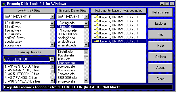
    Sure, the Giebler and Rubber Chicken utilities were still out there, but I’m a Mac guy, and attempts to get those running properly on emulated MS-DOS were pretty much a failure. What I needed was a utility that could read and write disk images on my Mac.

    A year ago I would have looked at that and said, “man, I do not have the time or the patience to read all those Transoniq Hacker articles and try to piece this together.” This year, I didn’t have to have that patience: I had Claude, and $20 worth of tokens a month to spend, so I thought, why not? This is actually a fairly well-defined problem:

    • Documentation for the disk organization and file formats exist in this PDF archive of the Transoniq Hacker
    • We have some disk images that we know work with the emulator, including a sequencer OS disk
    • The emulator seems to be able to read .IMG files fine, so if I can figure out how to write disks, I should be able to read them on the emulator.

    This is a pretty solidly mapped-out basis to start from, and I figured that with both good documentation, sample data, and a working system to test against, I stood a pretty good chance of being able to carefully steer Claude to a solution.

    Getting started

    I decided that I wasn’t going to be fancy here. This is going to be called sd1diskutil because it’s just going to be a wrapper around a library that knows how to do the job.

    So on March 26th, I sat down with Claude in the terminal, loaded obra/superpowers, and started brainstorming. I decided that, contrary to my more recent utility projects, I’d try to produce something that could be embedded into a prettier interface than just the command line.

    That meant the first decision was to what language to implement this in, and after some discussion with Claude, we settled on Rust, to allow me to make this a functional programming approach, using very tight types and operations on them. This was, in hindsight, probably colored by my experiences with Scala and really tight types, and how that made it so much easier to write correct code.

    To go with that and make it usable, we came up with a very thin CLI binary (sd1cli) that could convert MIDI SysEx dumps to and from the SD-1’s on-disk binary format provide full disk management — list, inspect, write, extract, delete, create.

    Because I knew that eventually I wanted to wrap this up in a pretty UI, I asked Claude how to build Swift bridging in, and it included a clean UniFFI surface for SwiftUI, allowing the same library to eventually power a macOS application.

    I knew that I was going to have to be very careful to implement this correctly. File systems and custom file formats are not forgiving, and the SD-1’s OS, though quite capable, is not what you would call robust.

    • The architecture therefore mirrored the data as closely as possible and tried to ensure that everything was as safe and stable as possible:
    • DiskImage owns the raw 819,200-byte image.
    • FileAllocationTable is a stateless handle that operates on a &mut DiskImage to avoid Rust borrow conflicts.
    • SubDirectory follows the same pattern.
    • SysExPacket is the only place nybble encoding and decoding happens — every layer above it works in plain bytes.
    • Atomic writes everywhere: save to a temp file, then rename.

    I started out with a blank disk template created by the SD-1 emulator. What better source for a good disk than the emulator itself? (Oh, you sweet summer child. We’ll spend about three days beating our heads against this disk image.)

    The first working implementation was achieved in a single burst: we planned out the types and operations, reviewed the design, and then built an implementation plan: workspace scaffold, error types, disk image, FAT, directory, SysEx parser, domain types, the full CLI. Integration tests for every command. The code compiled. The tests passed.

    Then came the reality checks.

    Block 4? Or block 5?

    The Giebler articles said that the FAT should be at block 5. But our empty disk image from the emulator said it was at block 4. Everything else matched up: ten blocks long, 170 three-byte entries each. What was the problem? We could write files with our code to the blank image, and the SD-1 emulator could read them.

    Figuring this took way longer than it should have, for a reason that only became clear in retrospect.

    The blank disk template used during early development, as mentioned above, had been written by the Sojus VST3 plugin, which it turned out was concealing a sector-shifting bug that was actually happening at the underlying MAME emulator level!

    See, normal DOS disks have 11 sectors per track, numbered 1 through 11. The SD-1 disks have ten, numbered zero to 9! MAME does handle the ten sectors per disk thing fine…but it uses SD-1 blocks 1 though 9, dropping block 0 and adding an empty all-zeroes block 10. So a fresh emulator-written disk has its FAT at block 4 instead of block 5. And a freshly-written emulator disk also immediately throws a DISK ERROR – BAD FORMAT if you try to read it…but we were only trying to write it, thereby breaking it, and then read it with our Rust code!

    The Giebler article in Transoniq Hacker said block 5 and our write code was written to put it at block 5, which was correct. The disk from the emulator said block 4, because the emulator dropped block 0. The emulator could read the test disks written by our code fine — because sd1diskutil‘s own writes were correct.

    But whenever the emulator saved a file back, it would quietly apply the shift again, moving the FAT back to block 4, exactly matching the initial (broken, but we didn’t know it) blank disk. So we went round and round, trying to resolve this: the article says 5, the disk says 4, the emulator reads 5 and writes 4, maybe both are correct and the article didn’t have that, so we should support either, or…?

    I repeatedly tried to add files to the disks written by the emulator, and they always got DISK ERROR – INVALID FORMAT. How was I screwing this up?

    I finally figured it out when I wrote a file to a good (block-5) disk and immediately tried to read it back (from the now block-4 disk). The emulator immediately threw a BAD DISK error…on its own output! So the emulator was wrong (though at the time we didn’t know why — see below!), and the article was right.

    We created an empty disk by taking a copy of the known-good SEQUENCER-OS disk and deleting all the files from it using our code. We then wrote a single file to it and tried it on the emulator…and the disk was readable and the file was there.

    Other early problems and fixes followed the same discipline of checking what we wrote against the emulator: local filenames needed to be forced to uppercase because the SD-1’s LCD doesn’t render lowercase. We had to analyze AllPrograms and AllPresets files on the SD-1 SEQUENCER-OS disk to figure out how to write them, and analyze how these were encoded into SysEx types (the SD-1 MIDI implementation helped some, but a lot had to be worked out from just trying things until we worked them out). The free block count management logic needed a rewrite. Each fix came from trying it and checking it against what the emulator would accept, not just blindly accepting the documentation, useful though it was,

    The Program Interleave Bug

    Of all the bugs, the program interleaving bug was the most insidious and hardest to fix, because it was wrong in a way that “worked”. Nothing broke, the OS didn’t complain, and on first glance seemed to be completely reasonable and perfectly correct…but sequences played back with all the wrong programs if they were being loaded from program memory. (ROM patches were fine.)

    Programs stored in a SixtyPrograms file are byte-interleaved on disk: there are two independent 15,900-byte streams packed together, with the even byte positions carrying programs 0 through 29, and the odd byte positions carrying programs 30 through 59.

    The original SysEx-to-program bank implementation had picked then outas alternating pairs — taking a program from the first half for bank 1, program 1, then a program from the second half for bank 1, program 2, and so on. The result was that programs were extracted perfectly, but landed at the wrong bank and patch position.

    I was able to figure this out by loading a custom 60-sequence file with 60 embedded programs, playing it back, and seeing that the expected patches were there but in the wrong places. Unfortunately, the fact that the last time I’d actually looked at these sequences was 2010 or so meant that I didn’t remember where the right position was! I knew they were wrong because they sounded wrong, but not where the right place was.

    It wasn’t until I found a SysEx dump of one of the factory sample sequences that we were able to write that to a .IMG and load it, then compare the locations where the programs went when our file was loaded in contrast to where they ended up when they were loaded from the SEQUENCER-OS disk by writing them down by bank and slot both ways and letting Claude figure out the mapping, which it did quite nicely.

    Extracting the even and odd byte streams in both the file we wrote and the “good” on-disk one, and then searching for known program names within each stream, allowed Claude to find where the one patch I definitely knew the sequence used was in both sets of interleaved data and then derive the correct mapping: a first-half/second-half split rather than alternating pairs.

    In the process of figuring all this out, we created a Python analysis tool, dump_programs.py, which could extract and list individual programs from multi-program SysEx dumps and disk files. Once we verified the extraction algorithm in the Python code, we were easily able to replicate it in Rust, and test it with two other sequence-and-program dumps by verifying they played back correctly on the emulator after being written to disk from a SysEx file.

    Sequences and a Deeper Problem

    Extracting sequences revealed a gap in the implementation: we could write SysEx files containing sequences and patches, but we couldn’t read them. There was a function that converted SysEx to the on-disk representation, but nothing that went the other direction.

    We discovered this when we realized that extraction was wrapping raw disk bytes in a SingleSequence SysEx header and producing output twice the expected size. Proper test-first setup allowed us to easily implement this properly, writing a 60-sequence-and-program file to disk, verifying it sounded correct on the emulator, and then reading it back out to .syx, verifying that the new file was a byte-for-byte match against the original.

    At this point, I wrote up the block-4/block-5 bug for the Sojus folks to take a look at on GitHub. (At this point I knew that there WAS a bug, but not WHY there was a bug.) They got back to me very quickly, and confirmed that yep, the emulator was screwing up the disk, and why.

    The plugin routes all floppy writes through MAME’s get_track_data_mfm_pc, a function that expects PC-standard sector numbering (1–10). As mentioned, the Ensoniq format uses 0–9. MAME silently discards sector 0 of every Ensoniq track, shifts the remaining sectors down by one, and zeros the last slot! Once the emulator rewrites the track, every block on the track contains wrong data, and every tenth block is zeroed. This was the same bug that had broken the early blank disk template and sent us chasing the wobbly FAT location for days — now fully understood, and confirmed with the Sojus developers, who identified the affected code as esq16_dsk.cpp in MAME — the DOS-to-Ensoniq-and-back block mapping.

    They’re busy working that as of 3/28, but in the meantime, they found a workaround: the emulation code can also read HFE format files. HFE stores the raw MFM flux data and bypasses MAME’s sector enumeration and extraction entirely. Which is totally awesome…but the sd1diskutil code did not speak HFE, and I’d never even heard of HFE. Watching the wonderful Usagi Electric suss out data encoding has educated me a little bit on data transitions and stuff like that, but it wasn’t something I was ready to work on myself at all!

    Archaeology Before Engineering

    Fortunately, the Sojus folks had an HFE image with some data on it to test with: two single patches (OMNIVERSE, SOPRANO-SAX) and a 60-program file. Claude and I embarked on trying to make sense of the data in this file, and this is where Claude seriously impressed me.

    We started off with this HFE file. We knew basically that it should have MFM data in it, and nothing else. Claude bootstrapped up from knowing what MFM data should look like to actually finding it in the file and making sense of this otherwise opaque stream of bits!

    Claude’s first attempt at locating sector headers found nothing. The standard MFM A1* sync marker should have been there ([0x44, 0x89]) but did not appear anywhere in the file. Claude figured out that this was because HFE stores bits LSB-first per byte, in the order the read head encounters them. The standard representation is MSB-first, so at first glance the data made no sense. Claude tried a bit-reversed version of the data, then a bit-reversed-per-byte version, and found the sync marker! [0x22, 0x91], with each byte bit-reversed.

    Once that hurdle was crossed, it was simple for Claude to find the markers and decode all 1600 sectors. The FAT free count in the decoded image matched the hardware OS block count: 1510. The block-to-sector mapping was confirmed against blank_image.img:

    block = track × 20 + side × 10 + sector

    Track geometry was pinned down: each side of a track is exactly 12,522 encoded bytes. The fixed preamble (Gap4a, sync, Gap1) consumes 284 bytes. Each of the 10 sectors is 1,148 bytes with a fixed structure. The remaining 758 bytes are inter-sector gaps — 75 bytes for sectors 0 through 8, and the rest absorbed by sector 9.

    I would have taken quite a long time and a lot of poring over the MFM spec and a lot of trial and error to figure this out, if ever, and Claude had it all doped out in half an hour or so.

    At this point Claude knew how to read an HFE file but not what we should do with it.

    We invoked the brainstorm/design spec/implemetation plan path again. I proposed that what we needed was a translation layer: just get the HFE image to an IMG image, and all of our tools could easily handle it. To use it on the emulator, we’d just convert the IMG image back to HFE, which the emulator should safely be able to read and write.

    Superpowers wrote a complete design spec before any Rust code was touched, pulling in all the information Claude already had at hand about how the HFE files work, writing Python code to cross-check assumptions made in the spec: exact constants, the complete MFM encoding rules, CRC16-CCITT coverage, the interleaved side storage layout, error variants, test cases, the works.

    Then superpowers wrote the implementation plan, with concrete function signatures, and specific expected outputs, all properly built as functions on types and easily testable.

    HFE Implementation, going full vibe

    At this point it was Claude’s party. I had read the spec and the plan, and everything looked reasonable, but I didn’t really know the HFE spec solidly enough to critique the code.

    Claude created three new error variants: InvalidHfe, HfeCrcMismatch, HfeMissingSector, each carrying track, side, and sector context so errors are never ambiguous. Then hfe.rs itself: 771 lines creating the full encode/decode pipeline, and new CLI subcommands hfe-to-img and img-to-hfe to encode and decode HFE images.

    The superpowers code review caught one bug: header offset 17 — the “do not use” field in the HFE v1 spec — was being written as 0x00. The spec requires 0xFF. A strict HFE reader would reject the file, and we knew the right answer, so…easy fix.

    After implementation, the code passed all the low-level tests, and read_hfe on the sample HFE file properly decoded all 1600 sectors, returning a DiskImage whose directory listed OMNIVERSE, SOPRANO-SAX, and 60-PRG-FILE with the correct free block count. A complete round-trip from .img to HFE and back produced a byte-for-byte identical result.

    The Acid Test

    The final test of the HFE pipeline started with the Sequencer OS disk: an 800K image containing every file type the SD-1 supports: Thirteen OneProgram files. Eleven SixPrograms banks. A ThirtyPrograms bank, eight SixtyPrograms banks, four TwentyPresets banks, eight sequence files of various sizes, and the sequencer OS binary itself (656,384 bytes!), totaling forty-nine files, and leaving just five free blocks.

    The disk was encoded to HFE and loaded into the emulator. Success! The emulator accepted the disk, an everything was present. I selected the sequencer OS, hit load, and it was loaded successfully. A previously-loaded sound bank in emulator memory contained a program named GREASE-PLUS, definitely not one already on the disk. I saved it to the HFE disk, and it wrote successfully.

    We decoded the modified HFE file to an IMG and listed the contents: fifty files. Three free blocks. GREASE-PLUS in disk slot 13, a OneProgram file, two blocks. Complete success!

    Future Plans

    Now that this is done, I plan to release it on GitHub as a library. If I get around to writing the pretty GUI, I will probably see if I can sell that, because why not? The Giebler disk utilities still sell for $60!

    At any rate, the CLI will be out there and should work, for anyone who wants to build it themselves.

  • Brachytheraphy, Pluvicto, and decay curves

    Earlier in the year, I had LDR (low-dose) brachytherapy treatment for prostate cancer. The way it works is that the radiation oncologist, in concert with the urologist/surgeon, maps out where the cancer is in the prostate, and then builds up a map in 3D of exactly where to implant a set of radioactive seeds to irradiate the cancer and as little as possible of other things, like the bladder, urethra, and colon.

    The treatment can use various radioactive isotopes; in my case, we decided on Palladium-103, which has a half-life of a tiny bit less than 17 days, and decays by electron capture, which I had not previously heard of.

    One of the K-shell electrons in palladium-103 has has a chance of having nonzero probability density inside the nucleus. (Think of a big cartoon sign pointing to the nucleus that says “YOU MIGHT BE HERE” for the electron.)

    If that happens, there’s a possibility that the weak nuclear force interaction between the electron and a proton in the nucleus will convert that proton into a neutron. That transforms the atom from palladium to rhodium and emits a neutrino.

    No big deal to emit a neutrino; billions of them are constantly sleeting through us every second from the sun. But! Now the rhodium atom is missing an electron in the K-shell, so one of the existing electrons drops into that shell and now the atom has excess energy to dump. One of two things happens:

    • The “we’ve all seen this one in physics class”: the atom emits a photon (in this case a low-energy X-ray), and we’re back to normal energy. Ho hum.
    • Then there’s the “you can do that?” option: the electrons just play “hot potato” and pass around the extra energy until one is bound loosely enough to be kicked out — this is an Auger electron (named after Pierre Victor Auger, though Lise Meitner published it a year earlier — the guys get the credit again); from the radiomedical standpoint, it acts as if it were a beta particle — it’s a high-energy electron — but doesn’t come from a nuclear decay: the electron is literally handed the excess energy and sent packing with it.

    For treating cancer, both of these are good news: the Auger electron is very short range but has high interactivity with the cancer cells to put them on the Oblivion Express (okay, that’s Brian Auger, not Pierre!); the X-ray photons travel further, but aren’t as strong. This means that the radioactivity is concentrated right where it’s needed.

    But it’s not 100% absorbed.

    One of the warnings I got was to make sure that I stayed around six feet away from young children and possibly-pregnant women for the first six weeks, as those are folks who can be affected much more by even the weak radioactivity I was shedding.

    That made me wonder: just how radioactive was I, compared to when I started? Let’s make a chart!

    Fortunately palladium-103’s decay is super simple: one path to rhodium-103, which is stable, so I can use the basic decay-curve equation to figure out exactly how much Pd-103 is left over time[1].

    N(t)=N0×e(λt)N(t) = N₀ × e^(-λt)

    This only requires us to know the decay constant λ, which we do: 16.99 days. We can plug that into a little Python program and get a nice curve:

    So the breakdown is actually pretty fast! We’re nearly at zero after 20 weeks, but because it’s an exponential curve, it’s a bit hard to read off numbers. Let’s look at that as a table:


     Weeks |  % Remaining
    ----------------------
    0.0 | 100.0000
    2.0 | 56.4887
    4.0 | 31.9097
    6.0 | 18.0254
    8.0 | 10.1823
    10.0 | 5.7519
    12.0 | 3.2492
    14.0 | 1.8354
    16.0 | 1.0368
    18.0 | 0.5857
    20.0 | 0.3308
    22.0 | 0.1869
    24.0 | 0.1056
    26.0 | 0.0596
    28.0 | 0.0337
    30.0 | 0.0190
    32.0 | 0.0107
    34.0 | 0.0061
    36.0 | 0.0034
    38.0 | 0.0019
    40.0 | 0.0011
    42.0 | 0.0006
    44.0 | 0.0003
    46.0 | 0.0002
    48.0 | 0.0001
    50.0 | 0.0001
    52.0 | 0.0000

    So at 6 weeks, the “it’s okay to stop warning people” cutoff, I’m at about 18% of the original intensity. That doesn’t give me an absolute number, but is interesting.

    I posted this on Reddit in r/ProstateCancer, just because it interested me; the mods did remove it, and fair, it’s more a curiosity than anything useful. Before it got pulled, though, I had one person ask me about how fast Pluvicto decayed — that’s Lutetium-177, and again, very fortunately a one-step-to-stable path. λ for Lu-177 is much shorter, about 6.4 days, so the curve falls off much faster:

    We’re pretty much at zero after ten weeks, which is significantly faster; the table looks like this:

     Weeks |  % Remaining
    ----------------------
    0.0 | 100.0000
    2.0 | 23.2255
    4.0 | 5.3943
    6.0 | 1.2528
    8.0 | 0.2910
    10.0 | 0.0676
    12.0 | 0.0157
    14.0 | 0.0036
    16.0 | 0.0008
    18.0 | 0.0002
    20.0 | 0.0000

    The warnings are different for Lu-177: “limit close contact (less than 3 feet) with household contacts for 2 days or with children and pregnant women for 7 days. Refrain from sexual activity for 7 days, and sleep in a separate bedroom from household contacts for 3 days, from children for 7 days, or from pregnant women for 15 days.”

    The remaining active Lu-177 is at about the same level, 20-ish percent in that amount of time, so my intuitive guess is that in terms of “radiation exposure to others”, the two are about the same.

    Pd-103 hangs around longer, but because it’s just dropping those Auger electrons and the low-energy X-rays, they don’t propagate as much, and the effect is much more localized.

    Lu-177 in Pluvicto circulates through the entire body, and binds to metastatic cancer cells there, so it makes sense that we’d want something that decayed a lot faster. (The Lu-177 decay is gamma and actual beta emission.)

    Conclusions? None really, it was simply trying to understand what was happening better, and was probably displacement activity. 🙂

    If you want to see the Python program that made the charts and tables, check out https://github.com/joemcmahon/decay_curve.

    [1] In college, I wrote my very first computer program to simulate the decay of a single U-235 atom to a stable state. I had learned about if statements and the rand() function, but not arrays. So I had a sheaf of if‘s that figuratively “ticked the clock” by one half life for each if block, moving on to the next when the random coin flip said the atom had taken another step along the decay path. It had all the structure and sophistication of a noodle.

    This was essentially a very bad and ridiculously unsophisticated Monte Carlo simulation, but in my defense, I had never written a computer program at all before, and I was extra proud I managed to make it work.

    There were a lot of long printouts of decay timelines on fanfold paper.

  • Using Perl to simulate a numbers station

    On the Disquiet Junto Slack, one of our members posted that they’d had a dream:

    I had a dream about a piece of gear last night. I wouldn’t say that it was “dream gear,” though it was still cool. It was a small black metal box, about the size of three DVD cases stacked on top of each other. There were a few knobs and sliders, a small 3-inch speaker, headphone out, and a telescoping antenna, so it kinda looked like a little radio at first. The antenna was there for radio reception but there was other stuff going on. It was intended to be used as a meditation/sleep aid/ASMR machine. There were sliders for a four-band EQ and a tuning knob for the radio. The tuning knob had a secondary function that tuned a drone sound (kinda sounded like a triangle wave fed through a wavefolder/resonance thinger). The other feature of this box was something like a numbers stations generator. Another slider was for the mix between the drone and a woman’s voice speaking random numbers and letters from the NATO alphabet in a Google Assistant-/Alexa-/Siri-type voice but with far less inflection. The four-band EQ was to be used like a mixer as well in that it was how a person could adjust how much of the radio signal was audible over the drone/numbers by using the output gain of the EQ. There was also a switch that fed the drone/numbers signal into the EQ as well. The EQ was intentionally low-quality so that when you took it above 0dB, it would distort.

    The Disquiet Junto Slack, #gear channel

    Now what was weird was that I’m been doing something like this in AUM; I had a quiet ambient Dorian sequence driven by ZOA on several instances of KQ Dixie (a DX7 emulator), and was using Radio Unit (a radio streaming AU) to layer in some birdsong. I realized I could mostly emulate the dream box if I added another Radio Unit to pull in some random stations, but generating the “numbers station” audio was more of a challenge – until I remembered that OS X has the say command, that will let you use the built-in speech synthesizers to pronounce text from the command line.

    I sat down, and after some fiddling (and looking up “how to add arbitrary pauses” so the rhythm was right), I created NATO::Synth to create the strings I wanted and pass them to say. It has a few nice little tweaks, like caching the strings created so it can decide to repeat itself, and properly inflecting the start and end of each “sentence”.

    I saved the generated audio (recorded with Audio Hijack) to iCloud, loaded it into AUM, and then recorded the results. Very pleased with it!

  • MVT under Hercules notes

    Update 12/2025: I finally found c3270, which is a usable if clunky 3270 emulator, so the changes to turn off 3270s are no longer needed. If, however, you find c3270’s PF key emulation a drag, go ahead and switch over to 3215’s.

    I also went through the whole MVT install process from zero and made a better version of the install guide. I’ll be posting that in my pages on this site in 2026, and saving a copy of a working MVT install to archive.org.

    • Full install of MVT with HASP and TSO
    • Verified that sysgen on the starter system works properly
    • Added some JCL to fix issues I had during the TSO install

    I needed a little mental relaxation this weekend, so I spent a while playing mainframe model trains by bringing up Hercules.

    I initially tried the MVS Turnkey system, but ran into some issues — mainly that there are no working (free) 3270 emulators for Big Sur. Since I couldn’t set up any consoles, and Homebrew x3270 didn’t seem to work under Xquartz, and I had no intention of spending $29 just to fool around with MVS for a bit, or multiple hours trying to get X11 builds working, I dropped back to Jay Maynard’s MVT installation instructions.

    They’re a bit out of date at the moment, and the Right Thing would probably be to make the fixes in both the instructions and the files, and move the corrected instructions over to a wiki somewhere. For now I’m leaving my notes here so I don’t forget what I did, and so I can do that later if I get the time. More fooling with the console and running jobs, less file twiddling.

    • You can get the OS/360 “CD-ROM” at http://www.jaymoseley.com/hercules/downloads/archives/os360mvt.tar.gz — this really ought to be on archive.org. It works with Maynard’s instructions and has these fixes:
      • dlibs/DN554.XMI was recovered. The srclibs/dn554 and related files in srclibs/TAPEFILE.ZIP have not been modified (recovered) to match, and should be at sone point.
      • srclib/fo520/IEYUNF.txt has been renamed to original.IEYUNF.txt and a version recovered from the MTS distribution has been added as IEYUNF.txt. The related file in srclibs/TAPEFILE.ZIP needs to be fixed as well.
      • These files are fine as they are to build MVT.
    • You need the JCL and HASP II tapes; they’re at http://www.conmicro.com/hercos360/os360ctl.tar.gz. Yes, I wish it was HASP IV, but I’m playing, so it’s not that big of a deal.
    • Maynard’s instructions are definitely of their time, when cutting and pasting commands was not a thing. The relevant commands are mentioned once, and one is expected to remember them. If I update these, I’ll inline the relevant command and note which console they get typed into. Switching back and forth between the Hercules “hardware” and the MVT console was a tad confusing at times. A significant omission: the devinit 00c foo.jcl command works okay for the MFT starter system and MVT without HASP, but once HASP is running the devinit must include eof at the end of the command or the reader hangs and the job never starts. Also, one of the HASP job filenames is called out by its right name in the section header, but by the wrong one in the text. Looks like a cut and paste error.
    • You should comment out or remove the 3270 definition at 0C0 in the mvt.cnf Hercules config file; if it’s there when you boot MVT, but no 3270 emulator is connected to it, the machine will hang with wait state 21. Took some googling to find that. TCAM will grumble about it when it starts up, but it doesn’t hurt anything.
    • You will need to install telnet on your Mac, since Big Sur removes it. telnet localhost 3270 to connect the virtual 3215 console. It might be worth trying to configure some 3215s for TSO and see if that works. We don’t really need to emulate real serial terminals.
    • Doing the mn jobnames, t and mn status commands will save you a lot of wondering whether anything is going on or not, even after HASP is up.
    • Be sure to copy the prt00e.txt virtual printer text file when:
      • You’ve finished doing both stages of the sysgen on the MFT system.
      • You’ve finished installing HASP.
      • You’ve finished installing TCAM and TSO

    Otherwise you lose all those useful assembler outputs of the HASP hooks and the TSO interfaces to it. The sysgen and TCAM build output isn’t critical, but it’s nice to have.

    Other things — http://hercstudio.sourceforge.net/ is supposed to be a hardware console emulator (lights and dials and stuff) interface for OS X and Linux; it’s written in Qt, which is fine, but the Makefile that qmake builds works to build it, but wants to install things in /usr/bin and Big Sur will not let it go there even with sudo. I might consider just writing a native iOS one instead.

    I’m up a couple hours later than I intended, but I have my notes, and as Adam Savage says, “the difference between science and screwing around is writing it down!”

  • obliquebot returns

    Some time back, when beepboop.com was still around, I wrote a little Slack bot that listened for “oblique” or “strategy” in the channels it had been invited to, and popped out one of Eno’s Oblique Strategies when it heard its keywords or was addressed directly.

    It worked fine up until the day that BeepBoop announced that they were going away, and eventually obliquebot stopped working.

    This month, I decided that I would stop ignoring the “you have a security issue in your code” notifications from GitHub, and try catching obliquebot up with the new version of the SLAPP library that I’d used to get Spud, the RadioSpiral.net “who’s on and what’s playing” robot back online.

    I went through all the package upgrades and then copied the code from Spud over to the obliquebot checkout. The code was substantially the same; both are bots that listen to channels and respond, without doing any complex interaction. I needed to add the code to load the strategies from a YAML file and to select and print one, but the code was mostly the same.

    I also needed to update the authentication page to show the obliquebot icon instead of the RadioSpiral one, and to set the OAuth callback link to the one supplied by Slack.

    Once I had all that in place, I spent a good two or three hours trying to figure out why I could build the code on Heroku, but not get it to run. I finally figured out that I had physically turned off the dyno, and that it wasn’t going to do anything until I tuned it back on again.

    obliquebot is now running again at RadioSpiral and the Disquiet Junto Slack, and I’ve updated the README at the code’s GitHub page to outline all the steps one needs to take it and build one’s own simple request-response bot.

  • Squaring numbers and a forgotten book

    I happened on a demonstration of a mental math trick on Reddit for squaring numbers in your head and was immediately reminded of a technique I learned in 1972 from a great book on speed arithmetic that I have unfortunately forgotten the name of.

    The video’s formulation uses the identity n^2 = (n^2 - a^2) + a^2 to make the multiplication simpler, but the book had an extremely elegant way to notate a different identity that works nicely for doing the squares of two-digit numbers in one’s head, and rapidly doing multi-digit squares on paper.

    The Reddit example squared 32 by changing it to 32 * 32 = 30 * 34 + 4 = 1024, which is clever, but check this out!

    Start with the identity (a + b)^2= a^2 + 2ab + b^2 and treat 32 * 32 as (30 + 2)^2.

    Visualize this in your head:

    0904 
     12

    That’s the a^2 + b^2 on the first line, and 2ab on the second. Now just add it up normally, with blank spaces equal to zeroes, and you get 0, 10, then 102, then 1024.

    The left-to-right add means you never have to remember the carry value, just the changed result. Let’s try 47.

    1649
     56

    1, 21, 220, 2209. Simple.

    The Wikipedia page on mental arithmetic is a great resource that has this technique, but lacks the notation visualization shown here which honestly is what makes it easy. The same technique works for larger numbers too. There’s more to remember, which may make it too hard to do in your head, but it makes squaring large numbers on paper trivial.

    Let’s say we want to square 123:

    010409 
     0412 
      06

    1, 14, 151, 1512, 15129. (a^2 + b^2 + c^2 + 2ab + 2bc + 2ac). Squares on the top row, 2ab on the left in the middle, 2bc on the right in the middle, 2ac on the bottom.

    I will admit that I didn’t properly get how to do the multi-digit notation right 45 years ago, but I hadn’t really understood the mapping of the identity to the positions on the page and was doing it by rote. The notation is the slickest part of this, as it automatically handles the proper number of multiplications by 10 for you.

    The left-to-right addition and a trick of doing mental addition by repeating the current total to oneself when adding the next number to keep from losing one’s place (ex. 45 + 37 + 62 – 45, 75, 75…82, 142, 144 and cast out 9s — 0, 1, 9, and 1+4+4 =9) were all also in that same book. I really wish I could remember what it was!

  • When did world computing power pass the equivalent of one iPhone?

    [This was originally asked on Quora, but the result of figuring this out was interesting enough that I thought I’d make it a blog post.]

    It’s a very interesting question, because there are so many differing kinds of computing capability in that one device. The parallel processing power of the GPU (slinging bits to the display) and the straight-ahead FLOPs of the ARM processor.

    Let’s try some back of the envelope calculations and comparisons.

    The iPhone 5’s A6 processor is a dual-core, triple-GPU device. The first multiprocessor computer was the Burroughs D-285 (defense-only, of course).

    Burroughs D-285

    A D-285 had 1 to 4 processors, running at ~ .070 s /1 operation = ~14 FLOPS for divide, the slowest operation, 166 FLOPS for add, the fastest, and ~25 FLOPS for multiply. Let’s assume adds are 10x more frequent than multiply and divide to come up with an average speed of 35 FLOPS per processor, so 70 FLOPS for a 2-processor D825, handwaving CPU synchronization, etc.

    Let’s take the worst number from the Geekbench stats via AnandTech for the iPhone 5’s processor: 322 MFLOPS doing a dot product, a pure-math operation reasonably similar to the calculations being done at the time in 1962. Note that’s MFLOPS. Millions. To meet the worst performance of the iPhone 5 with the most optimistic estimate of a 2-processor Burroughs D825’s performance, you’d need 4.6 million of them.

    I can state confidently that there were not that many Burroughs B362s available in 1962, so there’s a hard lower bound at 1962. The top-end supercomputer at that point was probably the IBM 7090, at 0.1 MFLOPS.

    #IBM 7090 Data Processing System / 1960 | Computer history, Computer generation, Old technology

    We’d still have needed 3200 of those. in 1960, there were in total about 6000 computers (per IBM statistics – 4000 of those were IBM machines), and very few in the 7090 range. Throwing in all other computers worldwide, let’s say we double that number for 1962 – we’re still way behind the iPhone.

    Let’s move forward. The CDC 7600, in 1969, averaged 10 MFLOPS (with hand-compiled code, and could peak at 35 MFLOPS).

    CDC-7600

    Let’s go with the 10 MFLOPS – to equal a single iPhone 5, you’d need 32 of them. Putting aside the once-a-day (and sometimes 4-5x a day) multi-hour breakdowns, we’re in the realm of possibility that the CDCs in existence alone at that time could equal or beat an iPhone 5 (assuming they were actually running), so the likelihood is that all computing in the world probably easily equalled or surpassed an iPhone 5 at that point in straight compute ability, making 1969 the top end of our range.

    So without a lot of complicated research, we can narrow it down to somewhere in the seven-ish years between 1962 and 1969, closer to the end than the start. (As a note, the Cray-1 didn’t make the scene till 1975, with a performance of 80 MFLOPS, a quarter of an iPhone; in 1982, the Cray X-MP hit 800 MFLOPS, or 2.5 iPhones.)

    And we haven’t talked about the GPUs, which are massively parallel processors the likes of which were uncommon until the 1980’s (and even the top-end graphics machines of the time 1962-1969 era couldn’t equal the performance of the iPhone’s GPU with weeks or months to work on rendering – let alone there not being output devices with the pixels per inch of the iPhone’s display capable of responding in real time). But on the basis of raw compute power, somewhere after the Beatles and before the moon landing. Making a finer estimate, I’d guess somewhere in late 1966, so let’s call it somewhere around the last Gemini mission, or Doctor Who’s first regeneration.

    On rereading the question I saw that the asker wanted the numbers for an iPhone 4 instead of a 5. Given the amount of handwaving I’m doing anyway, I’d say we’re still talking about close to the same period but a bit later. Without actual numbers as to the computers in use at the time, which I don’t think I can dig up without much more work than I’m willing to do for free, it’s difficult to be any closer than a couple years plus or minus. Definitely before Laugh-In (1968), definitely after the miniskirt (1964).

    iPhone 5s update: the 5s is about 1.75 times faster than the 5, so that puts us at a rough 530 MFLOPS. The computing power estimate becomes much harder at this point, as minicomputers start up about 1969 (the PDP-11 and the Data General Nova). The Nova sold 50,000 units, equivalencing out to about 130 MFLOPS; total PDP-11’s sold “during the 1970’s” was 170,000 for a total of 11 GFLOPS (based on the 11/40 as my guess as to the most-often-sold machine); divide that by ten and then take half of that for a rough estimate, and the PDP-11s by themselves equivalence to one 5s. So I’ll say that the moon landing was probably about the equivalence point for the 5s, but the numbers are much shakier than they are for the 4 or 5, so call it around the first message sent over ARPANet at the end of October 1969. (Side note: this means that the average small startup in Silicon Valley today – 20 or so people –  is carrying about the equivalent power of all the PDP-11’s sold during the 1970’s in their pockets and purses.)

    Past this, world computing power is too hard to track without a whole lot of research, so take this as the likely last point where I can feel comfortable making an estimate.